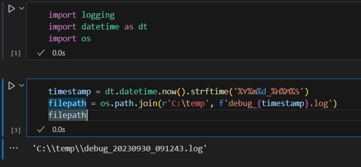
I will use the SQL Server online compiler for this post to display SQL. You can paste the SQL code in the window and run it to see results.
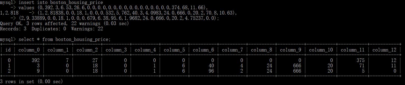
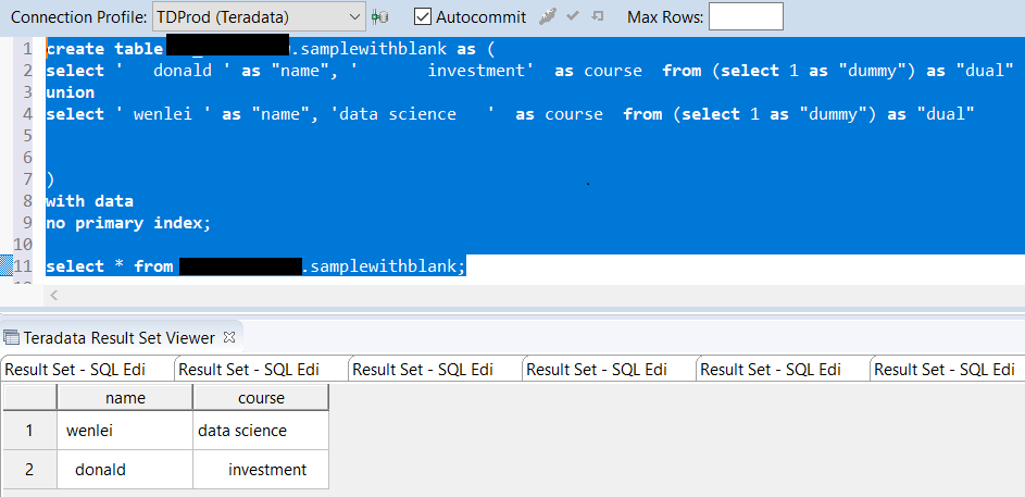
Let us first create a toy dataset. I use union to create a temp table, which will be used to demo what the results are supposed to be in SQL and compare with pandas results, which I will show in the Jupyter notebook.
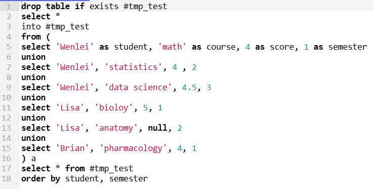
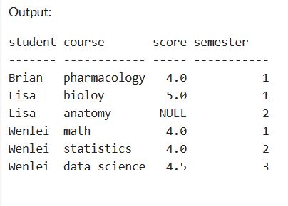
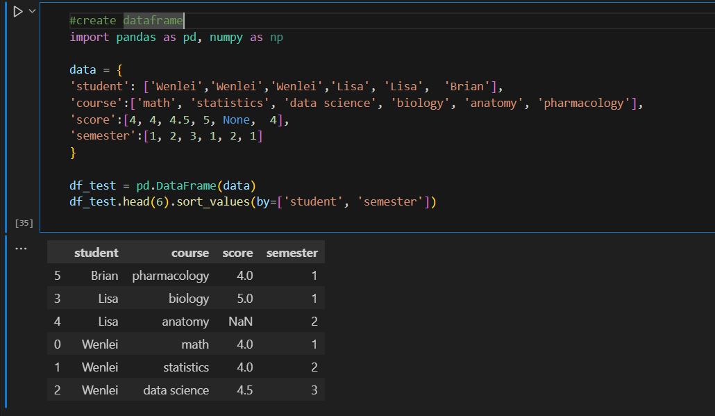
I deliberately include the null value here so that we can observe how SQL and pandas handle it. Pandas creates a dataframe which behaves like tables in a database.
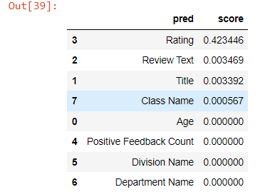
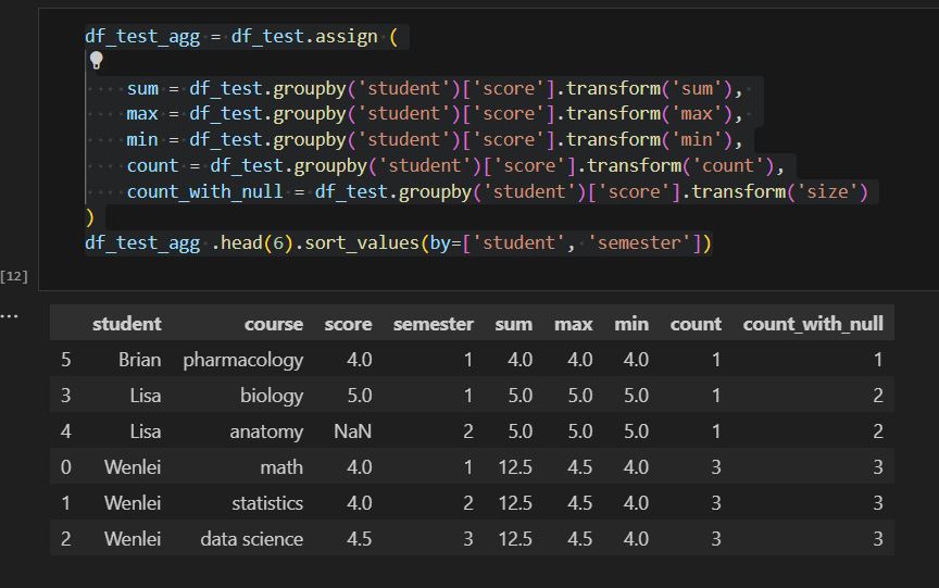
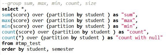
- The first challenge is using regular aggregation like sum/avg. With over (partition by …) SQL syntax, this allows us to get aggregation at each original row without reducing the row number like group by. This will help when you need to calculate different metrics in situ but don’t want to reduce the record. I have count(score) and count() here. The former will ignore null value in the score column, but count() will return all record counts.
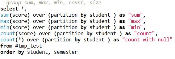
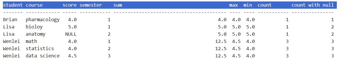
This can be achieved in pandas by groupby and transform function, Notice when you need to incude null, you will need to use size function instead.
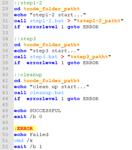
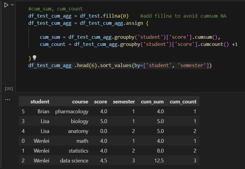
- Another form of aggregation is cumulative aggregation. In SQL, you will need to add sequence via order by, so that SQL engine knows how to combine data sequentially.
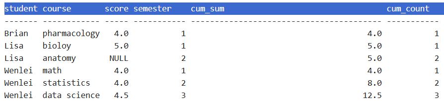
Because data contains null value, if we simply aggregate in pandas, null+number will end up with null. To fix that, we will need to fillna first, then we can use pandas cumsum and cumcount to get the result, because cumcount starts with 0, we will need to add 1 to match the results on the SQL side.
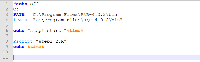
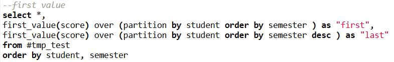
- Sometimes, we need to find the first or last record in one group, based on the certain sequence. This can be achieved by the first_value function combined with different order as follows.
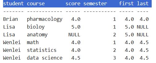
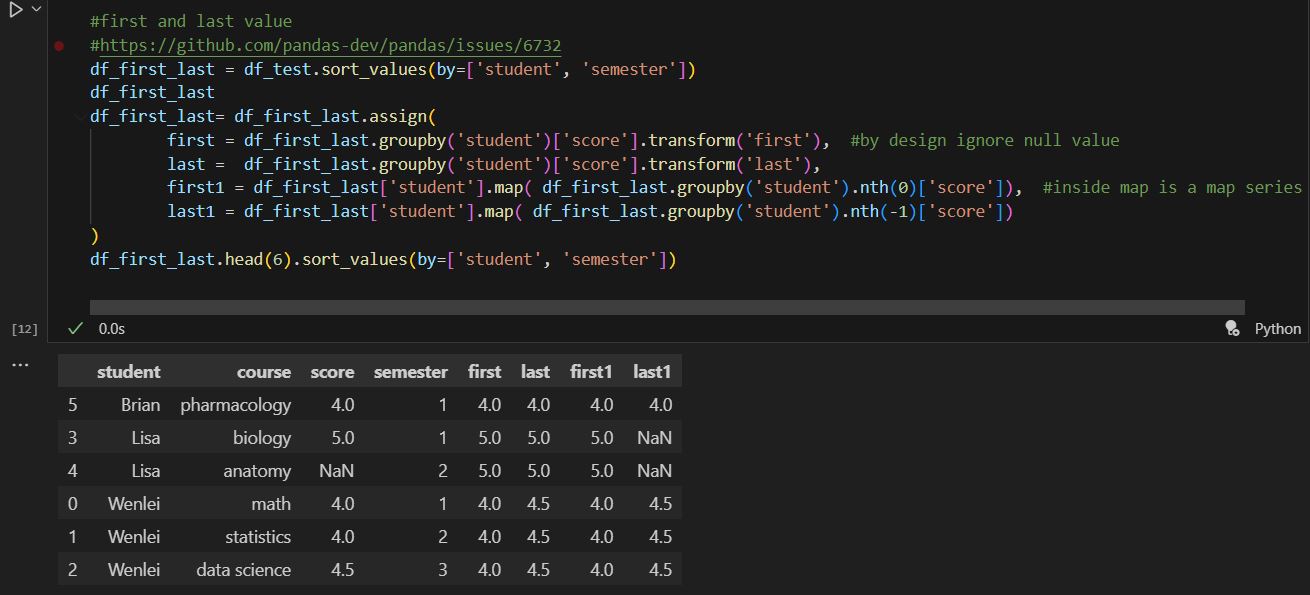
In pandas, it does have first and last functions, but unfortunately, it excludes the null value by default (see this github question). In order to simulate the same behavior in SQL, we will have to work around with the nth function which only works with groupby objects. The last two columns show the same behavior as SQL, inside map function, df_first_last.groupby(‘student’).nth(0)[‘score’] get the first score for each group. If we use nth(-1), that will be the last score.
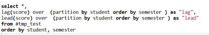
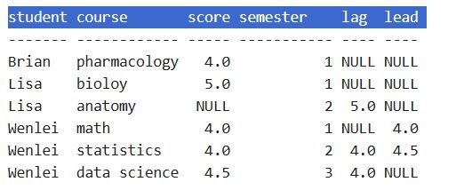
- Occasionally, you will need to compare the current record with other records in the same group. In SQL, you can use lead/lag. For e.g., you can do the following. Lag means to compare with the previous record depending on the sequence you set in the order by. Lead to get the next one.
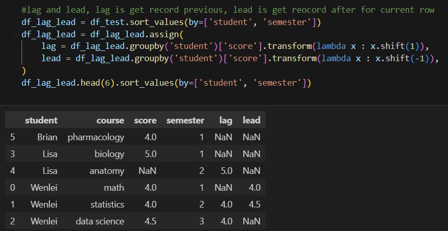
You can use transform and shift to achieve the same. Since we will need to pass in param, I use the lambda function here. Another thing to notice, I would think to use -1 to get the previous record, but in pandas, it uses 1 instead. sort of conterintuitive, but maybe developer think of the different way :))
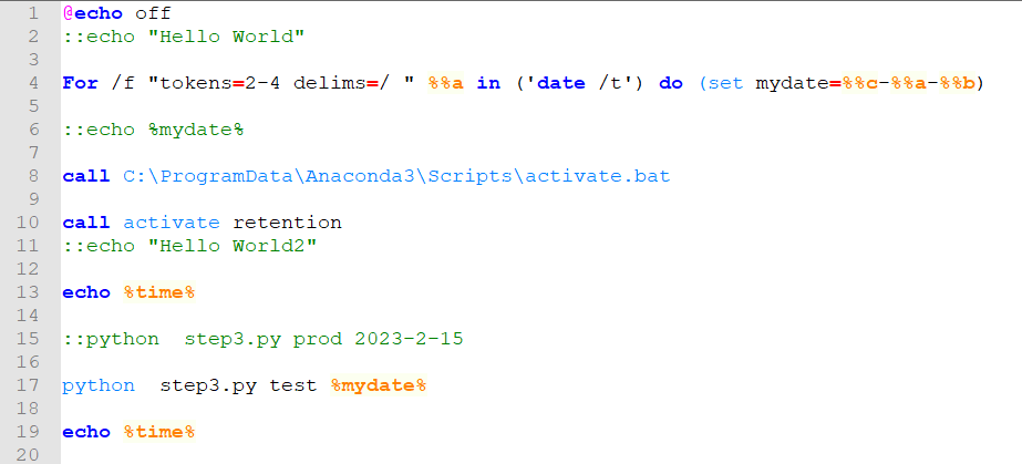
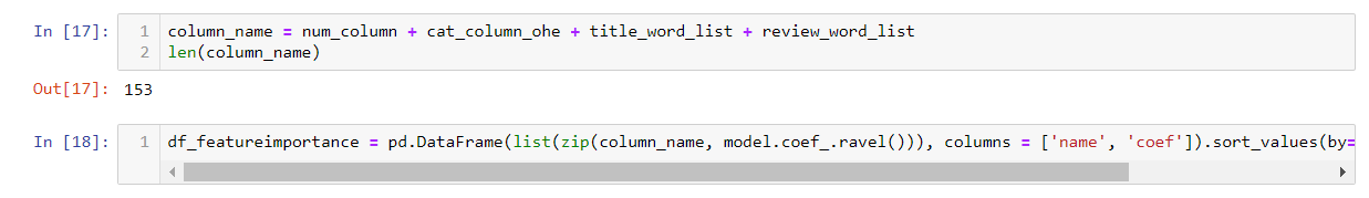
- It is not uncommon in real work, you will need to use row_number, rank, and dense_rank function among the same group to get sequence numbers. Row_nubmer will always give the different number even if value is equal, rank will give the same number if value is equal, but the sequence number will skip. Dense_rank is similar to rank, however, dense_rank will not skip the sequence number.
![]()
![]()
Obviously, I found a bug here in onecompiler.com marked by a red circle. It should be 2, 2, 1 since math and statistics are both 4.0. Pandas can handle this by using a rank function. Just notice, pandas rank ignore null value. if you need to include that, add na_option.
![]()
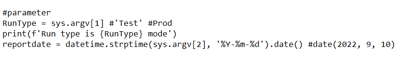
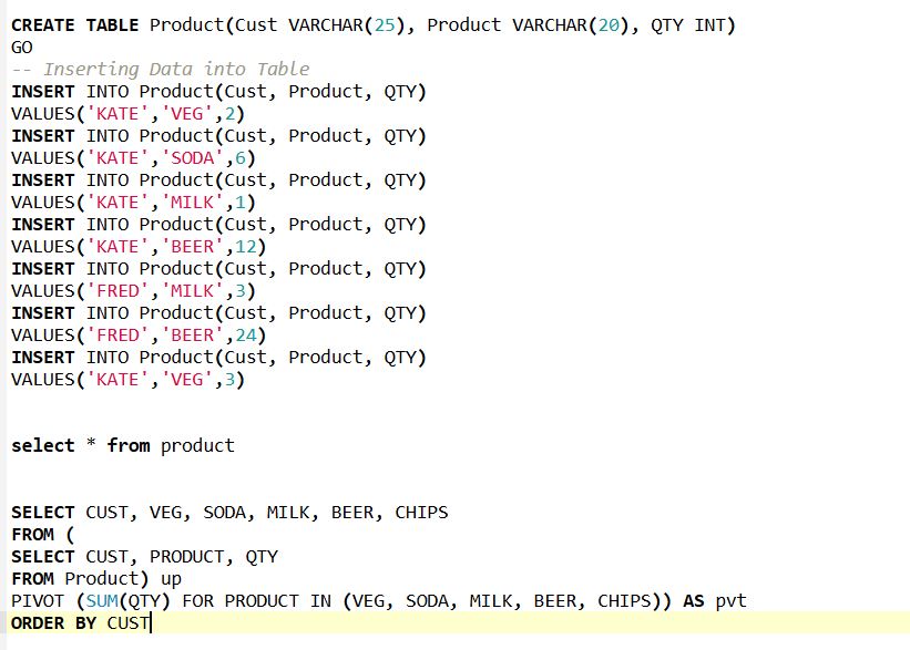
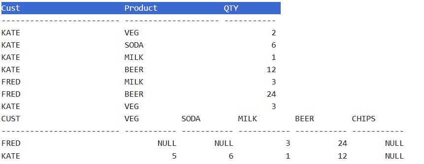
- You might come across a situation that requires you to pivot tables to get some insight. In SQL, you can use the pivot function. Here we created a separate table to demo this function. In the second part of results, you can see product column values have been pivoted to be column names. Also notice that you can list the column whatever you want. In this case, people add ‘chip’, which is not in the value of the original product, but it works just fine. In addition, some database recently included more rank functions, such as percent_rank which is used to let you know where the record stands percentage wise, but there is no corresponding function yet on the pandas side, I have tried different ways, so far, no luck yet, but I include the stack overflow discussion if you would like to give a shot.
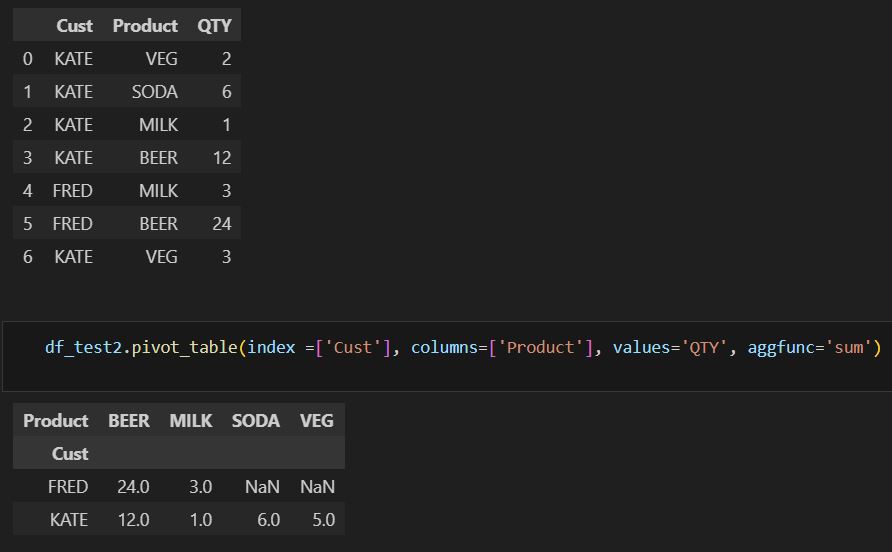
We create a df_test2 dataframe containing the same data. We can use pivot_table function to tell what I wound like on the row and column and what would be the value to be aggregated and what method I would like to aggregate (mean, sum, et al). Notice, there is no way you can insert “chips” here. Also, pivot_table has a sister function called pivot. Pivot_table can handle multiple columns. That is why you see the parameter is passed in as a list. Pivot can only handle one column at a time.
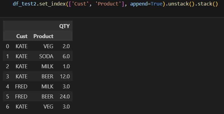
Pandas also offer a function to pivot row to column without aggregation. In this case, you will need to use unstack and stack functions. You will need to set index to the column you would like to pivot. By default, it will pivot the inner layer. But you can use the level parameter to adjust. You can reverse the unstack with the stack function.

in summary, pandas as a powerful open source tool has been able to achieve the vast majority of what database can offer. Although the implementation method could be slight different. for e.g., handling null value. so, be mindful.
I hope you feel this post is helpful. As usual, you can find the zip file containing both notebook and sql code file here.
you can also see result of sql here. but I don’t know how long they keep this link live https://onecompiler.com/sqlserver/42exn3g9w
thanks
Wenlei
]]>